latex Tutorial: How to plot Axes and Center of Symmetry

Greetings and welcome to yet another maths related Latex Tutorial. When graphing a function, it's often useful to plot the axes and center of symmetry as reference points. In this tutorial, we'll go over how to plot the axes and center of symmetry for two different functions:

$f(x) = 0.67(x-4)^2+1$

$g(x) = \sin(x) + 1$

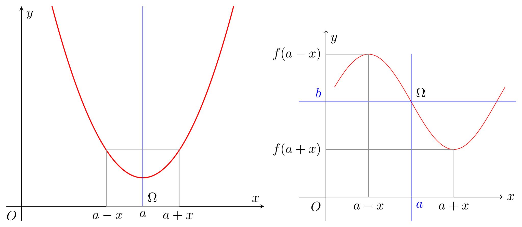
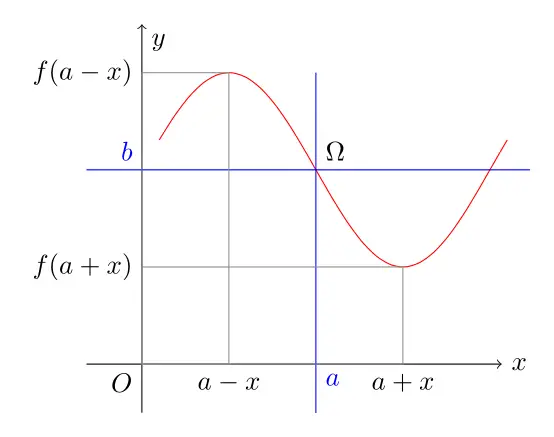
Plotting the Axes of Symmetry for $f(x)$

The function $f(x)$ is a quadratic polynomial of degree 2, with a leading coefficient of 0.67. The graph of the function $f(x) = 0.67(x-4)^2 +1$ is a parabola with a vertex at the point (-b/2a,f(-b/2a)) and an axes of symmetry of the equation: x = -b/2a. this is the axes that we need to plot alongside the parabola. the following Latex code will de just that

   
\begin{tikzpicture}[scale=0.50]
    \begin{axis}[axis lines=center,
	xlabel={$x$},
	ylabel={$y$},
	xtick=\empty,ytick=\empty,
	xmin=-0.5,xmax=8,
	ymin=-0.5,ymax=7,
	unbounded coords=jump,
	samples=200]
	\coordinate (A) at (2.8,0);
	\coordinate (B) at (5.2,2);
	\addplot [red,thick,domain=1:7.7,unbounded coords=jump]
	{0.67*(x-4)^2+1};
	\draw[blue] (4,0) -- (4,7) ;
	\draw[thin, gray] (A) rectangle (B) ;
	\node[below right] at (4.5,0) {$a+x$};
	\node[below ] at (4,0) {$a$};
	\node[below left ] at (0,0) {$O$};
	\node[above right ] at (4,0) {$\Omega$};
	\node[below left] at (3.5,0) {$a-x$};
     \end{axis}
\end{tikzpicture}
    

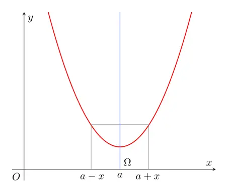
Plotting the Center of Symmetry for $g(x)$

The second function is a sinusoidal function of the form $g(x) = \sin(x)+1$. the y-shift is just to make the illustration look good. The function has a center of symmetry at the point Ω(π,1)

   
\begin{tikzpicture}[scale=0.65]
    \begin{axis}[axis lines=none,
	xlabel={$x$},
	ylabel={$y$},
	xtick=\empty,ytick=\empty,
	xmin=-2.5,xmax=7,
	ymin=-1.5,ymax=3,
	unbounded coords=jump,
	samples=200]
	\coordinate (A) at (0,2);
	\coordinate (B) at (0.5*pi,-1);
	\coordinate (C) at (0,0);
	\coordinate (D) at (1.5*pi,-1);
	\draw[->, black] (-1,-1) -- (6.5,-1) node[right] {$x$} ;
	\draw[->, black] (0,-1.5) -- (0,2.5) node[below right] {$y$} ;
	\draw[scale=1,domain=0.1*pi:2.1*pi,smooth,variable=\x,red] plot ({\x},{sin(\x r)+1});
	\draw[blue] (pi,-2) -- (pi,2) ;
	\draw[blue] (-1,1) -- (8,1) ;
	\draw[thin, gray] (A) rectangle (B) ;
	\draw[thin, gray] (C) rectangle (D) ;
	\node[below ] at (B) {$a-x$};
	\node[below right, blue ] at (pi,-1) {$a$};
	\node[below ] at (D) {$a+x$};
	\node[left ] at (A) {$f(a-x)$};
	\node[left ] at (C) {$f(a+x)$};
	\node[above left,blue ] at (0,1) {$b$};
	\node[above right ] at (pi,1) {$\Omega$};
	\node[below left ] at (0,-1) {$O$};
     \end{axis}
\end{tikzpicture}
    

And there you have it. until the next tutorial, happy editing and Plotting